Processing pipeline details

fMRIPrep adapts its pipeline depending on what data and metadata are available and are used as the input. For example, slice timing correction will be performed only if the SliceTiming metadata field is found for the input dataset.

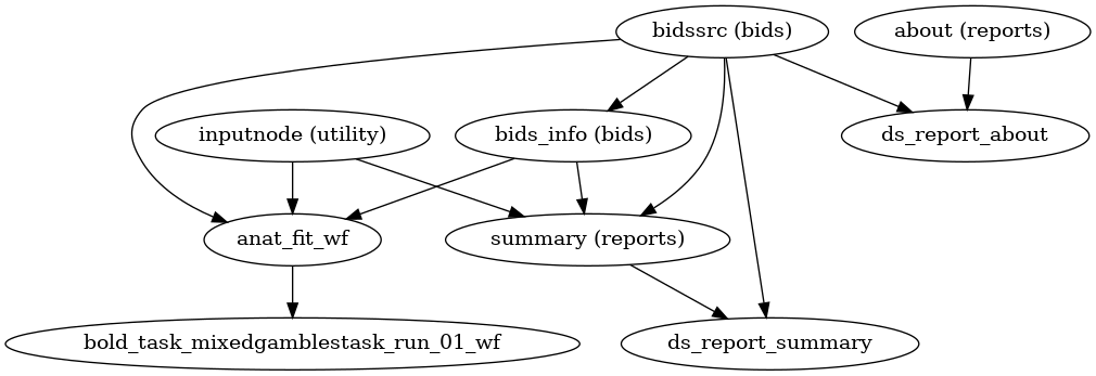
A (very) high-level view of the simplest pipeline (for a single-band dataset with only one task, single-run, with no slice-timing information nor fieldmap acquisitions) is presented below:

(Source code, png, svg, pdf)

Note

Each node in this workflow is either a processing node or a sub-workflow. Several conventions appear in this workflow that will be apparent throughout fMRIPrep.

• inputnodes are special nodes that provide the runtime-generated inputs to a workflow. These are like function “arguments”. There are corresponding outputnodes in most other workflows, which are like function return values.

• Workflows end with _wf, and are generated by a function of the form init_{workflow}_wf. For example, anat_preproc_wf is a sub-workflow that is generated by the init_anat_preproc_wf() (see below). Because each task and run of functional data is processed separately, init_bold_wf() names the resulting workflows using input parameters, resulting in func_preproc_task_{task}_run_{run}_wf.

• Datasinks begin with ds_, and save files to the output directory. This is in contrast to most nodes, which save their outputs to the working directory. ds_report_ nodes indicate that the node is saving text and figures for generating reports, rather than processed data.

• When a name appears in parentheses, such as (reports) in about (reports) it is the module where the interface is defined. In this case, about is an AboutSummary, found in the fmriprep.interfaces.reports module.

Preprocessing of structural MRI

The anatomical sub-workflow begins by constructing an average image by conforming all found T1w images to RAS orientation and a common voxel size, and, in the case of multiple images, averages them into a single reference template (see Longitudinal processing).

(Source code)

Important

Occasionally, openly shared datasets may contain preprocessed anatomical images as if they are unprocessed. In the case of brain-extracted (skull-stripped) T1w images, attempting to perform brain extraction again will often have poor results and may cause fMRIPrep to crash. fMRIPrep can attempt to detect these cases using a heuristic to check if the T1w image is already masked. This must be explicitly requested with ---skull-strip-t1w auto. If this heuristic fails, and you know your images are skull-stripped, you can skip brain extraction with --skull-strip-t1w skip. Likewise, if you know your images are not skull-stripped and the heuristic incorrectly determines that they are, you can force skull stripping with --skull-strip-t1w force, which is the current default behavior.

See also sMRIPrep’s init_anat_preproc_wf().

Brain extraction, brain tissue segmentation and spatial normalization

Then, the T1w reference is skull-stripped using a Nipype implementation of the antsBrainExtraction.sh tool (ANTs), which is an atlas-based brain extraction workflow:

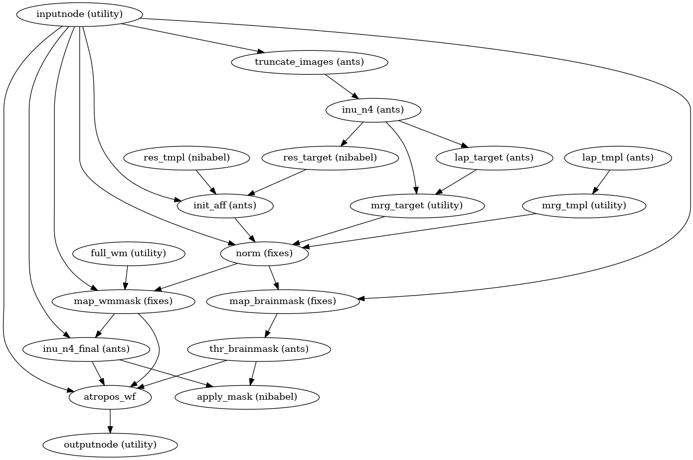
(Source code, png, svg, pdf)

Once the brain mask is computed, FSL fast is utilized for brain tissue segmentation.

fMRIPrep includes a single figure overlaying the brain mask (red), and tissue boundaries (blue = gray/white; magenta = tissue/CSF):

Brain extraction and segmentation report

Finally, spatial normalization to standard spaces is performed using ANTs’ antsRegistration in a multiscale, mutual-information based, nonlinear registration scheme. See Defining standard and nonstandard spaces where data will be resampled for information about how standard and nonstandard spaces can be set to resample the preprocessed data onto the final output spaces.

Animation showing spatial normalization of T1w onto the MNI152NLin2009cAsym template.

Cost function masking during spatial normalization

When processing images from patients with focal brain lesions (e.g., stroke, tumor resection), it is possible to provide a lesion mask to be used during spatial normalization to standard space [Brett2001]. ANTs will use this mask to minimize warping of healthy tissue into damaged areas (or vice-versa). Lesion masks should be binary NIfTI images (damaged areas = 1, everywhere else = 0) in the same space and resolution as the T1w image, and use the _roi suffix, for example, sub-001_label-lesion_roi.nii.gz. This file should be placed in the sub-*/anat directory of the BIDS dataset to be run through fMRIPrep. Because lesion masks are not currently part of the BIDS specification, it is also necessary to include a .bidsignore file in the root of your dataset directory. This will prevent bids-validator from complaining that your dataset is not valid BIDS, which prevents fMRIPrep from running. Your .bidsignore file should include the following line:

*lesion_roi.nii.gz

Note

The lesion masking instructions in this section predate the release of BIDS Derivatives. As of BIDS 1.4.0, the recommended naming convention is:

manual_masks/
└─ sub-001/
   └─ anat/
      ├─ sub-001_desc-tumor_mask.nii.gz
      └─ sub-001_desc-tumor_mask.json

In an upcoming version of fMRIPrep, we will search for lesion masks as pre-computed derivatives. Until this is supported, we will continue to look for the _roi suffix.

Longitudinal processing

In the case of multiple T1w images (across sessions and/or runs), T1w images are merged into a single template image using FreeSurfer’s mri_robust_template. This template may be unbiased, or equidistant from all source images, or aligned to the first image (determined lexicographically by session label). For two images, the additional cost of estimating an unbiased template is trivial, but aligning three or more images is too expensive to justify being the default behavior. For consistency, in the case of multiple images, fMRIPrep constructs templates aligned to the first image, unless passed the --longitudinal flag, which forces the estimation of an unbiased template.

Note

The preprocessed T1w image defines the T1w space. In the case of multiple T1w images, this space may not be precisely aligned with any of the original images. Reconstructed surfaces and functional datasets will be registered to the T1w space, and not to the input images.

Surface preprocessing

fMRIPrep uses FreeSurfer to reconstruct surfaces from T1w/T2w structural images. If enabled, several steps in the fMRIPrep pipeline are added or replaced. All surface preprocessing may be disabled with the --fs-no-reconall flag.

Note

Surface processing will be skipped if the outputs already exist.

In order to bypass reconstruction in fMRIPrep, place existing reconstructed subjects in <output dir>/sourcedata/freesurfer prior to the run, or specify an external subjects directory with the --fs-subjects-dir flag. fMRIPrep will perform any missing recon-all steps, but will not perform any steps whose outputs already exist.

If FreeSurfer reconstruction is performed, the reconstructed subject is placed in <output dir>/sourcedata/freesurfer/sub-<subject_label>/ (see FreeSurfer derivatives).

Surface reconstruction is performed in three phases. The first phase initializes the subject with T1w and T2w (if available) structural images and performs basic reconstruction (autorecon1) with the exception of skull-stripping. Skull-stripping is skipped since the brain mask calculated previously is injected into the appropriate location for FreeSurfer. For example, a subject with only one session with T1w and T2w images would be processed by the following command:

$ recon-all -sd <output dir>/freesurfer -subjid sub-<subject_label> \
    -i <bids-root>/sub-<subject_label>/anat/sub-<subject_label>_T1w.nii.gz \
    -T2 <bids-root>/sub-<subject_label>/anat/sub-<subject_label>_T2w.nii.gz \
    -autorecon1 \
    -noskullstrip

The second phase imports the brainmask calculated in the Preprocessing of structural MRI sub-workflow. The final phase resumes reconstruction, using the T2w image to assist in finding the pial surface, if available. See init_autorecon_resume_wf() for details.

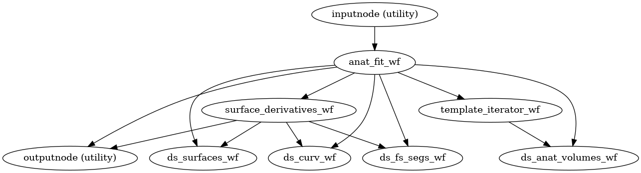
Reconstructed white and pial surfaces are included in the report.

Surface reconstruction (FreeSurfer)

If T1w voxel sizes are less than 1mm in all dimensions (rounding to nearest .1mm), submillimeter reconstruction is used, unless disabled with --no-submm-recon.

If T2w or FLAIR images are available, and you do not want them included in FreeSurfer reconstruction, use --ignore t2w or --ignore flair, respectively.

lh.midthickness and rh.midthickness surfaces are created in the subject surf/ directory, corresponding to the surface half-way between the gray/white boundary and the pial surface. The smoothwm, midthickness, pial and inflated surfaces are also converted to GIFTI format and adjusted to be compatible with multiple software packages, including FreeSurfer and the Connectome Workbench.

Note

GIFTI surface outputs are aligned to the FreeSurfer T1.mgz image, which may differ from the T1w space in some cases, to maintain compatibility with the FreeSurfer directory. Any measures sampled to the surface take into account any difference in these images.

(Source code, png, svg, pdf)

See also sMRIPrep’s init_surface_recon_wf()

Refinement of the brain mask

Typically, the original brain mask calculated with antsBrainExtraction.sh will contain some inaccuracies including small amounts of MR signal from outside the brain. Based on the tissue segmentation of FreeSurfer (located in mri/aseg.mgz) and only when the Surface Processing step has been executed, fMRIPrep replaces the brain mask with a refined one that derives from the aseg.mgz file as described in RefineBrainMask.

BOLD preprocessing

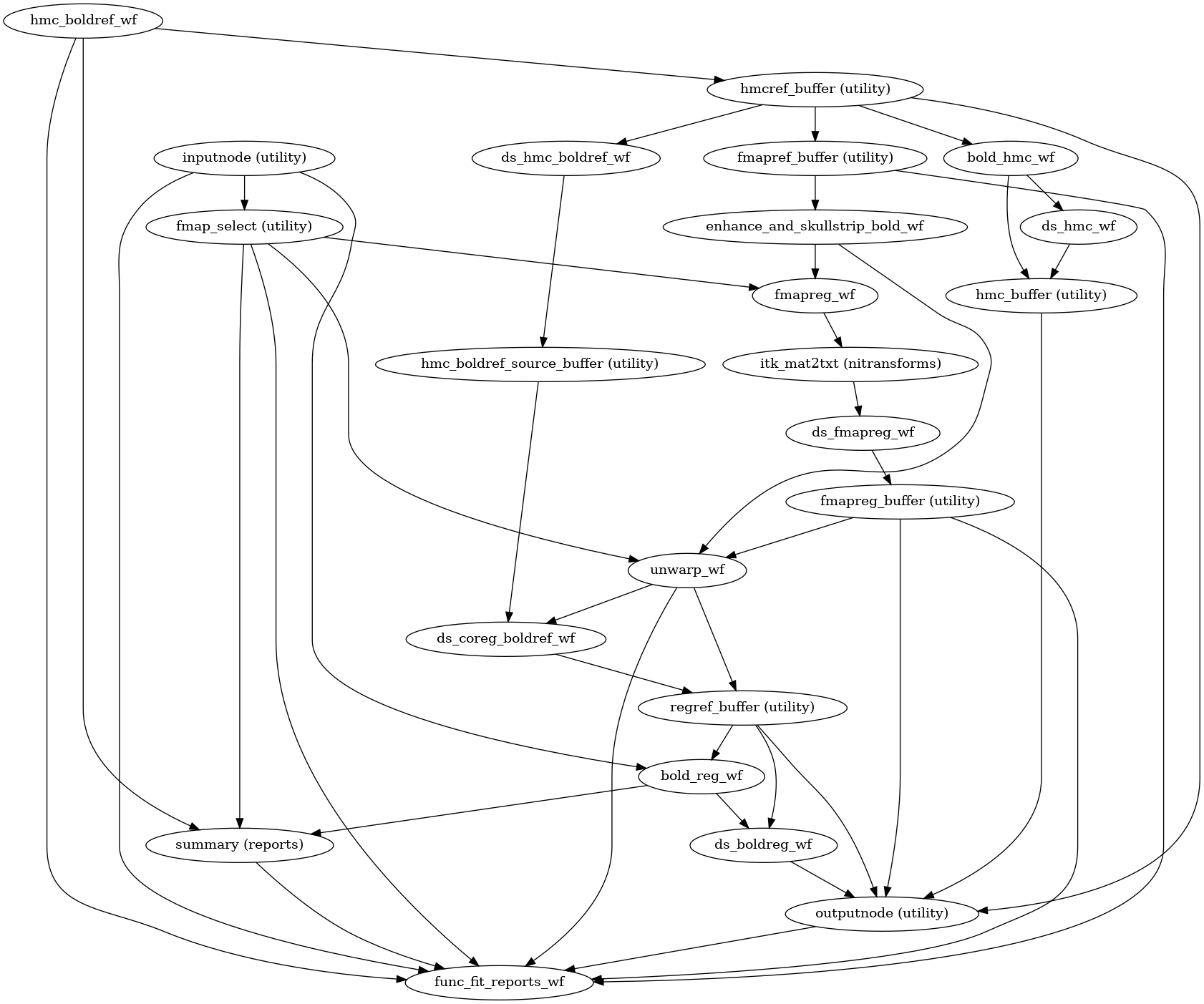
fMRIPrep performs a series of steps to preprocess BOLD data. Broadly, these are split into fit and transform stages.

The following figures show the overall workflow graph and the bold_fit_wf subgraph:

init_bold_wf()

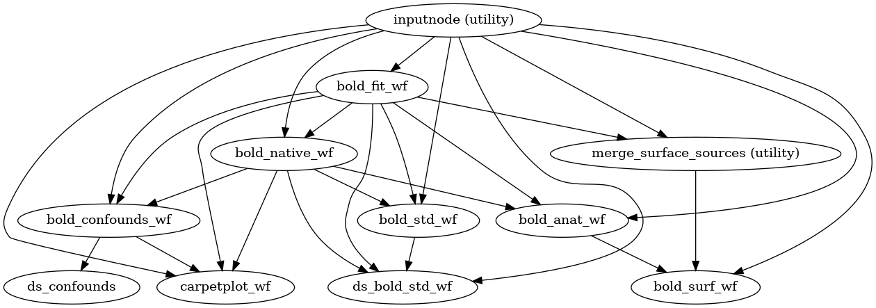
(Source code, png, svg, pdf)

init_bold_fit_wf()

(Source code, png, svg, pdf)

Preprocessing of BOLD files is split into multiple sub-workflows described below.

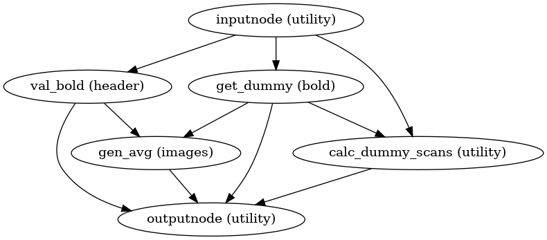
BOLD reference image estimation

init_raw_boldref_wf()

(Source code, png, svg, pdf)

This workflow estimates a reference image for a BOLD series as follows: When T1-saturation effects (“dummy scans” or non-steady state volumes) are detected, they are averaged and used as reference due to their superior tissue contrast. Otherwise, a median of motion corrected subset of volumes is used.

This reference is used for head-motion estimation.

For the registration workflow, the reference image is either the above described reference image or a single-band reference, if one is found in the input dataset. In either case, this image is contrast-enhanced and skull-stripped (see init_enhance_and_skullstrip_bold_wf()). If fieldmaps are present, the skull-stripped reference is corrected prior to registration.

The red contour shows the brain mask estimated for a BOLD reference volume. The blue and magenta contours show the tCompCor and aCompCor masks, respectively. (See Confounds estimation, below.)

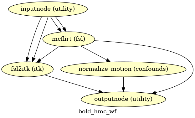
Head-motion estimation

init_bold_hmc_wf()

(Source code, png, svg, pdf)

Using the previously estimated reference scan, FSL mcflirt is used to estimate head-motion. As a result, one rigid-body transform with respect to the reference image is written for each BOLD time-step. Additionally, a list of 6-parameters (three rotations, three translations) per time-step is written and fed to the confounds workflow. For a more accurate estimation of head-motion, we calculate its parameters before any time-domain filtering (i.e., slice-timing correction), as recommended in [Power2017].

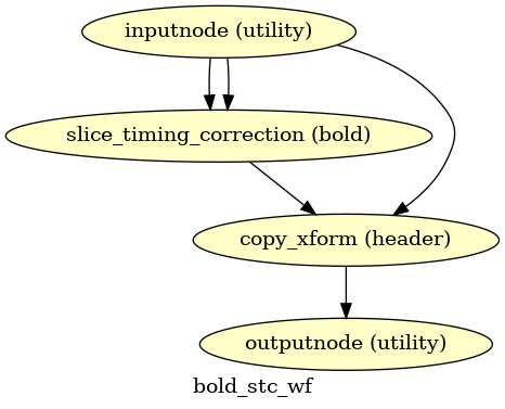
Slice time correction

init_bold_stc_wf()

(Source code)

If the SliceTiming field is available within the input dataset metadata, this workflow performs slice time correction prior to other signal resampling processes. Slice time correction is performed using AFNI 3dTShift. All slices are realigned in time to the middle of each TR.

Slice time correction can be disabled with the --ignore slicetiming command line argument. If a BOLD series has fewer than 5 usable (steady-state) volumes, slice time correction will be disabled for that run.

Susceptibility Distortion Correction (SDC)

One of the major problems that affects EPI data is the spatial distortion caused by the inhomogeneity of the field inside the scanner.

Applying susceptibility-derived distortion correction, based on fieldmap estimation.

Please note that all routines for susceptibility-derived distortion correction have been excised off of fMRIPrep for utilization on other projects (e.g., dMRIPrep). For more detailed documentation on SDC routines, check on the SDCFlows component.

Theory, methods and references are found within the SDCFlows documentation.

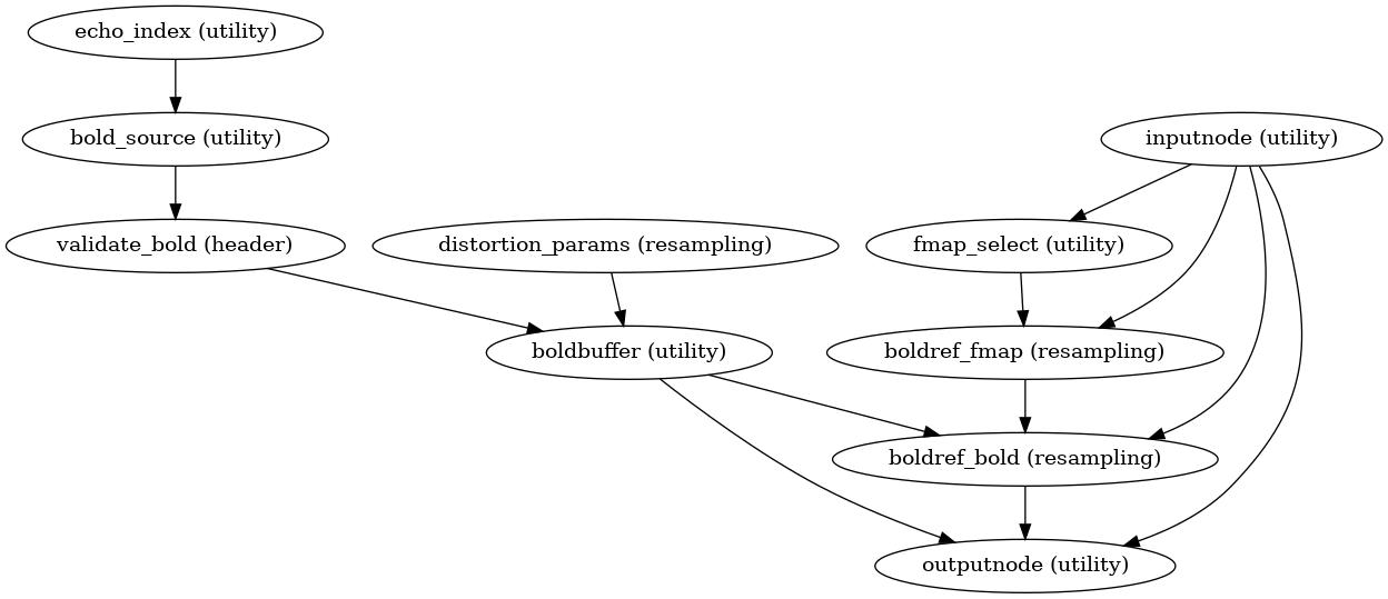
Pre-processed BOLD in native space

init_bold_native_wf()

(Source code, png, svg, pdf)

A new preproc BOLD series is generated from the slice-timing corrected or the original data (if STC was not applied) in the original space. All volumes in the BOLD series are resampled in their native space by concatenating the mappings found in previous correction workflows (HMC and SDC if executed) for a one-shot interpolation process. Interpolation uses a Lanczos kernel.

EPI to T1w registration

init_bbreg_wf()

(Source code, png, svg, pdf)

The alignment between the reference EPI image of each run and the reconstructed subject using the gray/white matter boundary (FreeSurfer’s ?h.white surfaces) is calculated by the bbregister routine. See fmriprep.workflows.bold.registration.init_bbreg_wf() for further details.

Animation showing EPI to T1w registration (FreeSurfer bbregister)

If FreeSurfer processing is disabled, FSL flirt is run with the BBR cost function, using the fast segmentation to establish the gray/white matter boundary. See fmriprep.workflows.bold.registration.init_fsl_bbr_wf() for further details.

After either BBR workflow is run, the resulting affine transform will be compared to the initial transform found by FLIRT. Excessive deviation will result in rejecting the BBR refinement and accepting the original, affine registration.

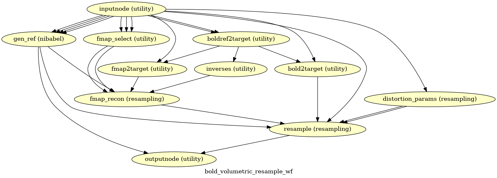
Resampling BOLD runs onto standard spaces

init_bold_volumetric_resample_wf()

(Source code)

This sub-workflow concatenates the transforms calculated upstream (see Head-motion estimation, Susceptibility Distortion Correction (SDC) –if fieldmaps are available–, EPI to T1w registration, and an anatomical-to-standard transform from Preprocessing of structural MRI) to map the EPI image to the standard spaces given by the --output-spaces argument (see Defining standard and nonstandard spaces where data will be resampled). It also maps the T1w-based mask to each of those standard spaces.

Transforms are concatenated and applied all at once, with one interpolation (Lanczos) step, so as little information is lost as possible.

The output space grid can be specified using modifiers to the --output-spaces argument.

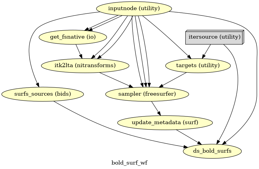
EPI sampled to FreeSurfer surfaces

init_bold_surf_wf()

(Source code, png, svg, pdf)

If FreeSurfer processing is enabled, the motion-corrected functional series (after single shot resampling to T1w space) is sampled to the surface by averaging across the cortical ribbon. Specifically, at each vertex, the segment normal to the white-matter surface, extending to the pial surface, is sampled at 6 intervals and averaged.

Surfaces are generated for the “subject native” surface, as well as transformed to the fsaverage template space. All surface outputs are in GIFTI format.

HCP Grayordinates

init_bold_fsLR_resampling_wf()

(Source code)

If CIFTI output is enabled, the motion-corrected functional timeseries (in T1w space) is resampled onto the subject-native surface, optionally using the HCP Pipelines_’s “goodvoxels” masking method to exclude voxels with local peaks of temporal variation. After dilating the surface-sampled time series to fill sampling holes, the result is resampled to the fsLR mesh (with the left and right hemisphere aligned). These workflows make use of various Connectome Workbench functions. These surfaces are then combined with corresponding volumetric timeseries to create a CIFTI-2 file.

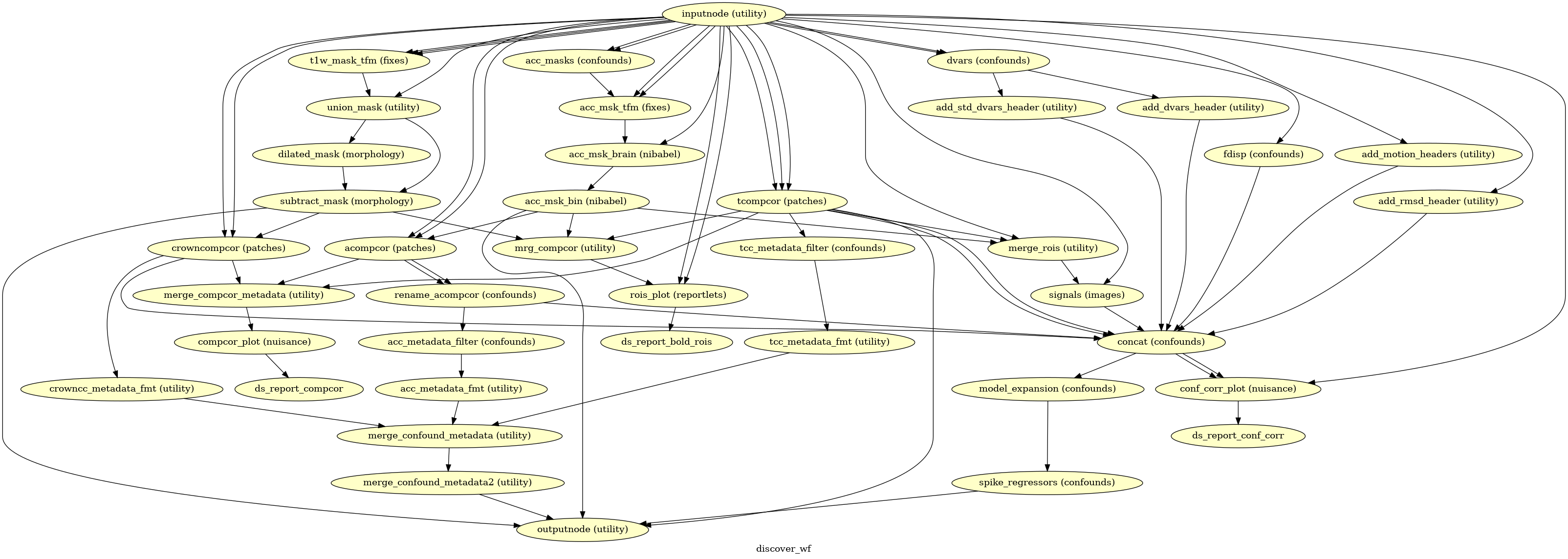
Confounds estimation

init_bold_confs_wf()

(Source code, png, svg, pdf)

Given a motion-corrected fMRI, a brain mask, mcflirt movement parameters and a segmentation, the discover_wf sub-workflow calculates potential confounds per volume.

Calculated confounds include the mean global signal, mean tissue class signal, tCompCor, aCompCor, Frame-wise Displacement, 6 motion parameters, DVARS, and spike regressors.

T2*-driven echo combination

init_bold_t2s_wf()

(Source code, png, svg, pdf)

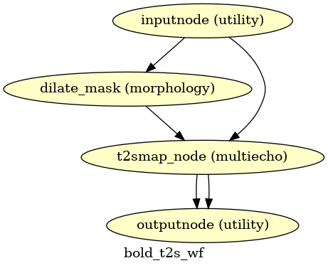
If multi-echo BOLD data is supplied, this workflow uses the tedana T2* workflow to generate an adaptive T2* map and optimally weighted combination of all supplied single echo time series. This optimally combined time series is then carried forward for all subsequent preprocessing steps.

The method by which T2* and S0 are estimated is determined by the --me-t2s-fit-method parameter. The default method is “curvefit”, which uses nonlinear regression to estimate T2* and S0. The other option is “loglin”, which uses log-linear regression. The “loglin” option is faster and less memory intensive, but it may be less accurate than “curvefit”.

References

[Power2017]

Power JD, Plitt M, Kundu P, Bandettini PA, Martin A (2017) Temporal interpolation alters motion in fMRI scans: Magnitudes and consequences for artifact detection. PLOS ONE 12(9): e0182939. doi:10.1371/journal.pone.0182939.

[Brett2001]

Brett M, Leff AP, Rorden C, Ashburner J (2001) Spatial Normalization of Brain Images with Focal Lesions Using Cost Function Masking. NeuroImage 14(2) doi:10.006/nimg.2001.0845.